Introduction to Arrays

2.1. Introduction to Arrays#

An array is a sequence of values or objects. The values can be of any type, but it is very common with arrays of numbers (integers or floating point numbers), in which case the array can be used to present vectors, matrices, and tensors. The values in an array are often referred to as elements.

One way to create a so-called 1-d array (or a vector) is to list the elements, separated by commas, inside square brackets ([ ]):

x = [1, 2, 4, -3]

4-element Vector{Int64}:
  1
  2
  4
 -3

typeof(x)

Vector{Int64} (alias for Array{Int64, 1})

In the output we can see that the x variable has the type Vector{Int64}, and the typeof command reveals that this is actually just an alternative name for the more general array type Array{Int64,1}. Julia identified based on the elements that this appears to be an array of integers, and uses the default integer type Int64. The 1 in the Array form refers to the fact that this is a 1-d array (that is, a vector).

y = [1.1, π, -4/3, 1e-1]

4-element Vector{Float64}:
  1.1
  3.141592653589793
 -1.3333333333333333
  0.1

The y variable is also a vector, but since it contains floating point numbers Julia uses the default type Float64 for all of the elements.

You can also create an array with elements of a specified type using the following syntax:

z = Float64[1, 2, 4, -3]    # Without the `Float64`, Julia would make this an integer array

4-element Vector{Float64}:
  1.0
  2.0
  4.0
 -3.0

Arrays can also be created using built-in functions, such as the ones below where T indicates the type of the elements and defaults to Float64 if omitted:

Function	Description
`zeros(T, n)`	a vector of all zeros
`ones(T, n)`	a vector of all ones
`trues(n)`	a `BitArray` with all values `true`
`falses(n)`	a `BitArray` with all values `false`
`range(start, stop=stop, length=n)`	range of `n` linearly spaced elements from `start` to `stop`

Some other useful functions include the push! function, which adds a new element to the end of an array:

push!(z, 10)

5-element Vector{Float64}:
  1.0
  2.0
  4.0
 -3.0
 10.0

Note the exclamation mark ! at the end of the function name, it indicates that this function modifies some of its arguments (in this case the array z).

Similarly, the append! function adds the elements of the second array to the end of the first:

append!(z, y)

9-element Vector{Float64}:
0
0
0
 -3.0
0
1
141592653589793
 -1.3333333333333333
1

2.1.1. Accessing the elements of an array#

We can access an element in an array using an index inside square brackets. Julia arrays are 1-based, meaning that the indices start at 1. The keyword end can be used to refer to the last element of the array, and the function length(x) returns the number of elements in the array x.

y[3]   # Access the 3rd element in the array y

-1.3333333333333333

z[1] = z[end] * z[end-1]      # Set the 1st element in z to the product of the last two elements
z                             # To print the entire array

9-element Vector{Float64}:
 -0.13333333333333333
  2.0
  4.0
 -3.0
 10.0
  1.1
  3.141592653589793
 -1.3333333333333333
  0.1

2.1.2. Traversing an array#

A common operation is to traverse the elements of an array. This can be done using a for-loop with an index variable:

for i = 1:length(x)
    println("Element ", i, " of the array x has the value ", x[i])
end

Element 1 of the array x has the value 1
Element 2 of the array x has the value 2
Element 3 of the array x has the value 4
Element 4 of the array x has the value -3

An alternative syntax uses the in keyword, and does not need an index variable:

for element in x
    println("This element of x has the value ", element)
end

This element of x has the value 1
This element of x has the value 2
This element of x has the value 4
This element of x has the value -3

2.1.3. Example: Sieve of Eratosthenes#

The sieve of Eratosthenes is a simple, ancient algorithm for finding all prime numbers up to any given limit \(n\). From Wikipedia:

Create a list of consecutive integers from \(2\) through \(n\): \((2, 3, 4, ..., n)\).
Initially, let \(p\) equal \(2\), the smallest prime number.
Enumerate the multiples of \(p\) by counting in increments of \(p\) from \(2p\) to \(n\), and mark them in the list (these will be \(2p\), \(3p\), \(4p\), …; the \(p\) itself should not be marked).
Find the first number greater than \(p\) in the list that is not marked. If there was no such number, stop. Otherwise, let \(p\) now equal this new number (which is the next prime), and repeat from step 3.
When the algorithm terminates, the numbers remaining not marked in the list are all the primes below \(n\).

As a refinement, it is sufficient to mark the numbers in step 3 starting from \(p^2\), as all the smaller multiples of \(p\) will have already been marked at that point. This means that the algorithm is allowed to terminate in step 4 when \(p^2\) is greater than \(n\).

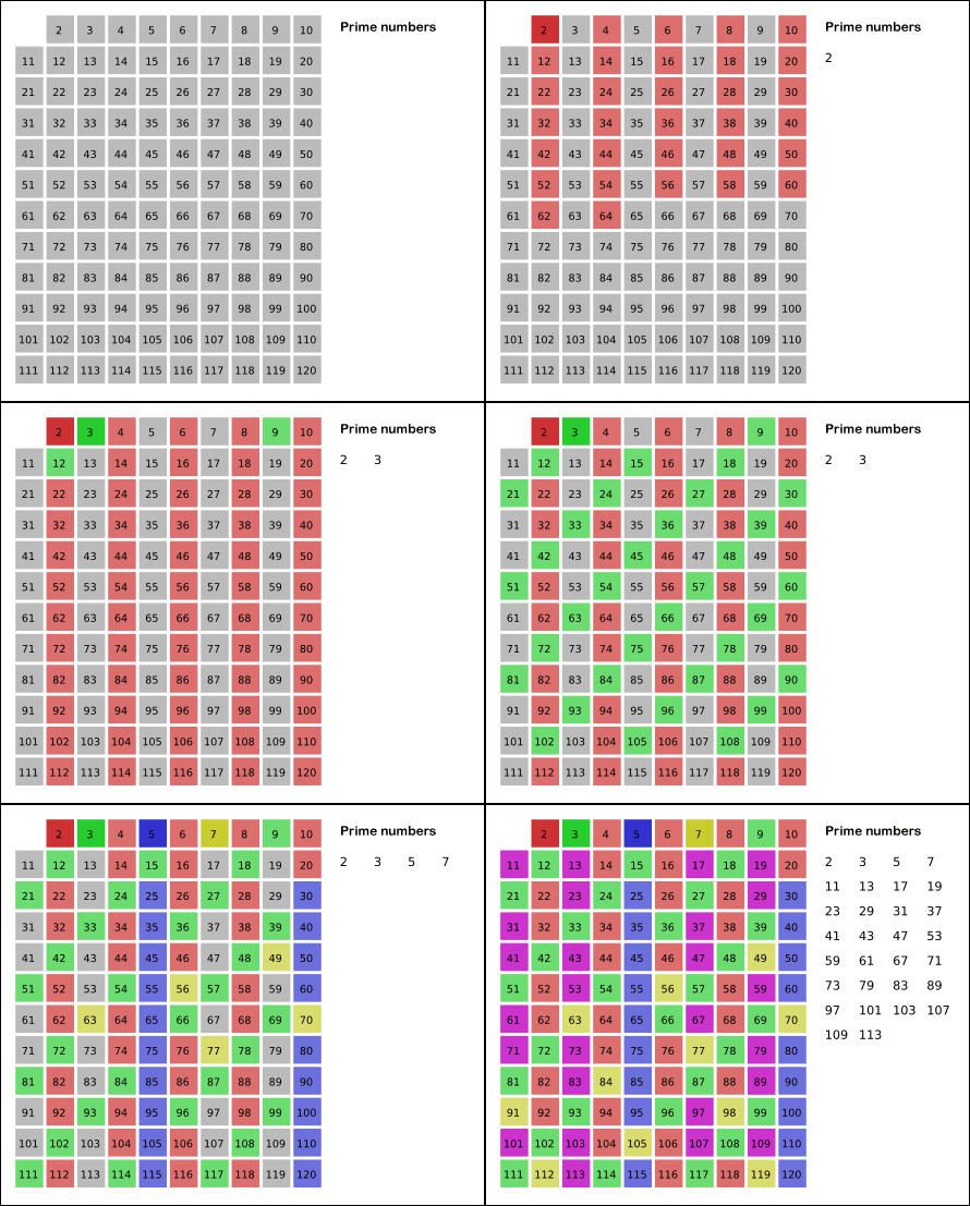
Wikipedia also provides an animation to illustrate the method:

Wikipedia Sieve of Eratosthenes animation

An implementation of the algorithm is shown below. The only remaining new function we need for this is the floor function, to find the largest integer such that \(p^2\le n\). This can be found using isqrt(n), which returns the largest integer less than or equal to \(\sqrt{n}\).

function SieveOfEratosthenes(n)
    # Create a boolean array of length n, initialize all entries to as true
    # After the algorithm finishes, prime[i] will be true is i≥2 is a prime
    prime = trues(n)
    
    for p = 2:isqrt(n)
        if prime[p]
            for i = p^2:p:n
                prime[i] = false
            end
        end
    end
    
    # Return an array with all prime numbers
    primes = Int64[]
    for i = 2:n
        if prime[i]
            push!(primes, i)
        end
    end
    primes
end

SieveOfEratosthenes (generic function with 1 method)

println(SieveOfEratosthenes(100))            # All prime numbers up to 100

[2, 3, 5, 7, 11, 13, 17, 19, 23, 29, 31, 37, 41, 43, 47, 53, 59, 61, 67, 71, 73, 79, 83, 89, 97]

println(SieveOfEratosthenes(1000000)[end])   # The largest prime number less than 1,000,000

2.1.4. The dot-syntax: Vectorized operators and functions#

Julia provides a convenient dot-syntax to perform element-by-element operations on an array.

For every binary operator, e.g. *, there is a corresponding dot operator .* which is automatically defined to perform the * operation element-by-element.
Any function f can be applied elementwise to an array by using the automatically defined function f.

These dot-operators are illustrated in the examples below.

x = [1, 3, 5]
y = [0.2, 4.0 , 3.1]
z = x .* y   # Element-by-element multiplication

3-element Vector{Float64}:
2
0
5

sqrt.(x)     # Element-by-element square roots

3-element Vector{Float64}:
0
7320508075688772
23606797749979

w = x .+ sqrt.(y .^ x)      # More complex mathematical expression, element-by-element

3-element Vector{Float64}:
4472135954999579
0
920151004054308

For elementwise complex expressions such as in the last example, Julia provides a @. syntax that makes all operators in the expression be applied elementwise:

@. x + sqrt(y^x)       # Same as before

3-element Vector{Float64}:
4472135954999579
0
920151004054308

When using the dot-operator on binary operations, the two arrays much have the same number of elements:

push!(y, 7)
x .* y      # Error: arrays must have same number of elements

DimensionMismatch: arrays could not be broadcast to a common size; got a dimension with lengths 3 and 4

Stacktrace:
 [1] _bcs1
   @ ./broadcast.jl:529 [inlined]
 [2] _bcs
   @ ./broadcast.jl:523 [inlined]
 [3] broadcast_shape
   @ ./broadcast.jl:517 [inlined]
 [4] combine_axes
   @ ./broadcast.jl:512 [inlined]
 [5] instantiate
   @ ./broadcast.jl:294 [inlined]
 [6] materialize(bc::Base.Broadcast.Broadcasted{Base.Broadcast.DefaultArrayStyle{1}, Nothing, typeof(*), Tuple{Vector{Int64}, Vector{Float64}}})
   @ Base.Broadcast ./broadcast.jl:873
 [7] top-level scope
   @ In[18]:2

However, if one of the arguments to the operator is a scalar, it is interpreted as a constant vector of the correct size:

x .* -3

3-element Vector{Int64}:
  -3
  -9
 -15

The dot-syntax also works as expected for numerical literal coefficients:

-3x

3-element Vector{Int64}:
  -3
  -9
 -15

Note that the dot-syntax is automatically defined even for new functions:

function pick_largest(x, y)
    if x > y
        return x
    else
        return y
    end
end

pick_largest (generic function with 1 method)

println("z = ", z)
println("w = ", w)
println("elementwise largest = ", pick_largest.(z,w))

z = [0.2, 12.0, 15.5]
w = [1.4472135954999579, 11.0, 21.920151004054308]
elementwise largest = [1.4472135954999579, 12.0, 21.920151004054308]

2.1.5. Array slices#

An array can be sliced, which means extracting a subset of the original array. This subset can be expressed as a range of indices, similar to the for-loop syntax, or more generally it can be any vector of integer indices.

println(y)               # Original vector
println(y[1:3])          # First 3 elements
println(y[1:2:4])        # All odd-numbered elements
println(y[end:-1:2])     # From end back to second element in reverse
println(y[4:3])          # Empty subset
println(y[:])            # All elements (same as original vector)
println(y[[4,2,4,3,3]])  # Index by vector - pick elements 4,2,4,3,3

[0.2, 4.0, 3.1, 7.0]
[0.2, 4.0, 3.1]
[0.2, 3.1]
[7.0, 3.1, 4.0]
Float64[]
[0.2, 4.0, 3.1, 7.0]
[7.0, 4.0, 7.0, 3.1, 3.1]

These so-called ranges can also be used to define the array itself. For example:

    x = 1:8

will define an object that can be used as an array. If needed, the matrix can be explicitly created using the collect function:

x1 = collect(1:3)

3-element Vector{Int64}:
 1
 2
 3

x2 = collect(10:-2.5:-3)

6-element Vector{Float64}:
0
5
0
5
0
 -2.5