Defining functions

Functions are just another type of expression in Mathematica

Their argument lists take the form of patterns. We will discuss patterns in more depth in the next lecture

For now, we will make use of one kind of pattern: x_
which matches any expression and calls it x.
For example:

This function can be called with any kind of argument. That argument will be called x in the body of the function, which gives a result by adding one

There are much more sophisticated patterns than just “match any expression.” We will cover these later.

Suppose we want to recursively compute the factorial
Base case: fac(0) = 1
Recursive definition: fac(n) = n*fac(n-1)

This is simple to define in Mathematica.
We begin with the base case

Now, fac[0] will evaluate to 1

We don’t have a rule for the general case, so fac[n] will remain unevaluated:

Defining the general case:

Let’s do a similar exercise with the Fibonacci sequence: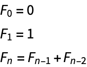

Of course, Mathematica also has this built in, so we can check our work...

Solving recurrence relations

Suppose we have the recurrence relation

We can easily create a function to recursively evaluate this sequence

What if we want to know a general (non-recursive formula)?
First, concentrate on the recursive definition (ignoring boundary conditions)
We can solve this recurrence by making the ansatz that is given by for some r
In that case,

So, we look for solutions to this equation.

So, r=5 and r=2 satisfy this relationship.
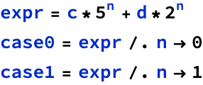
The general solution will be given by

We can easily solve the system of equations to find the values of c and d.
But we can also let Mathematica help...

Let’s check our formula

ClearAll deletes all the definitions we made for a

Mathematica can also solve the recurrence directly using RSolve

More complicated functions and local variables

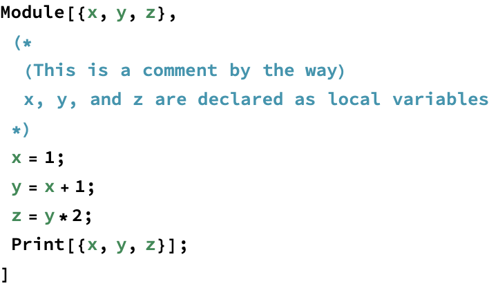
Sometimes we want to introduce local variables in a function for intermediate values in long calculations

This can be achieved using Module

Mathematica also has other scoping mechanisms (i.e. for creating variables with local scope)
See e.g. Block, With

For our uses, Module is sufficient

Functional style programming

Mathematica is a multi-paradigm programming language

It supports both functional and imperative programming, but functional constructs are often very natural

For example, applying a function f to a list is known as mapping f over the list

Map is considered so important in Mathematica it has its own syntax

We can define more complicated functions if we want

Sometimes we want to create an anonymous function so that we don’t need to name it

Here # indicates the argument, and & tells Mathematica that the preceding expression is a function

This notation can easily become hard to read, so be careful

More functional programming

Recall our list

We can apply filters to the list using Select

We can combine this with anonymous functions

Sometimes we want to apply a function to a list for its side-effect rather than its return-value

For this we have Scan

There are a ton more functional programming facilities in Mathematica

See e.g. Nest, Fold, Apply

Can we get the sum of all of these entries?

Patterns

We have seen one type of pattern before: x_

The underscore will match any expression, and then the result will be called x

We can test if a pattern matches an expression using MatchQ

There are other kinds of patterns.

Except will match anything except what’s in the brackets

You can match for specific heads of expressions with _h

Conditions can be added to a pattern with /;

Boolean functions can also be added with the ? operator

Patterns can be combined using | for or

Type checking

Checking for specific heads allows us to perform type checking

Let’s get rid of our old (overly-general) rule

We want to add a condition to the pattern: only match non-negative integers

Another example

Example: defining our own derivative function

We want to differentiate arbitrary expressions

This can be achieved using the basic rules of differentiation:

Linearity

Product rule

Chain rule

We first need the concept of an expression being independent of another expression.
This is achieved using FreeQ

Some common base cases:

Addition:

Scalar multiplication:

Product rule

Chain rule

(Have to be careful in the above not to match f[x] (so make sure g doesn’t match x), otherwise have infinite recursion)

If we encounter functions whose derivatives we don’t know, it will leave them unevaluated:

We can easily add rules for trigonometric functions:

Our definitions will automatically work with function composition:

Speed: memoization

Recall our Fibonacci sequence

How fast (slow?) is it?

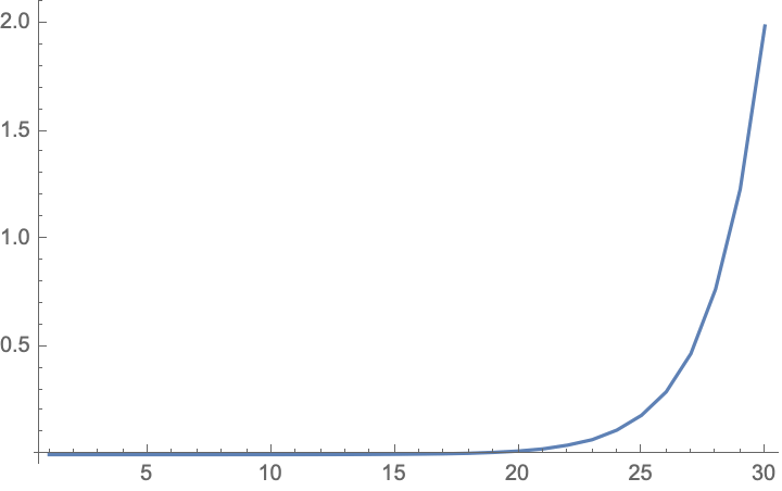
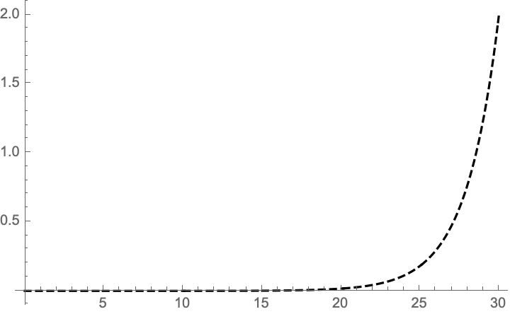
In fact, the runtime for the recursive algorithm satisfies

and so the time to compute fib[n] is actually given by fib[n]

We can easily find a closed form representation of the Fibonacci sequence (involving the golden ratio) using e.g. the characteristic polynomial

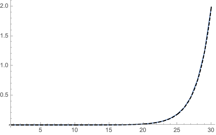
We can try to optimize our recursive implementation using memoization

Look how many times fib[1] and fib[0] are evaluated! We can speed things up by storing these values

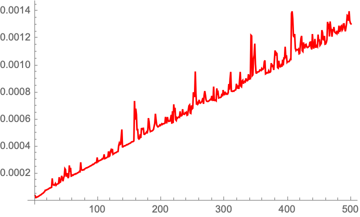
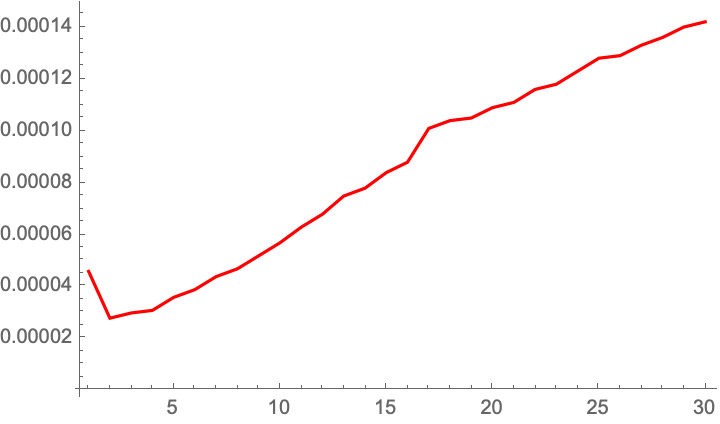
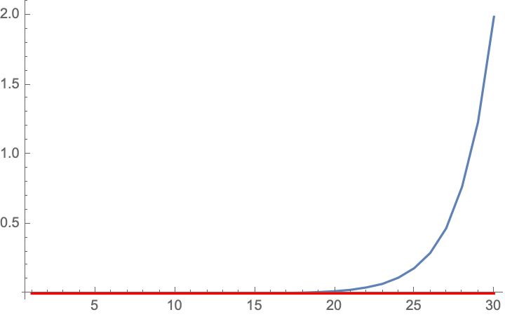
We can see that the timings are linear, which is clear given the recurrence