In the previous section, we discussed the distribution of eigenvalue gaps for Gaussian Ensembles. In particular, we showed Wigner's surmise was a reasonable approximation to the distirbution's density. In this section, we will demonstrate how to compute the true underlying distribution for GUEs and their connection to the zeros of the Riemann Zeta function.

Distribution of Spacings of Eigenvalue of GUEs

The density of the distribution of gaps between eigenvalues can be computed as the solution to the Painleve V ODE. We will follow the procedure prescribed by Alan Edelman and Per-Olof Persson in Numerical Methods for Eigenvalue Distribution of Random Matrices.

Painleve V

We say $\sigma$ satisfies the Painleve V differential equation if for $t > 0$

$$(t\sigma'')^2 - 4(\sigma - t\sigma')(t\sigma'-\sigma + (\sigma')^2) = 0 $$

with the boundary condition

$$\sigma(t) \approx -\frac{t}{\pi} - \left( \frac{t}{\pi} \right)^2 \ \text{ as } t \rightarrow 0^+$$

We can rewrite the ODE as

$$ \sigma'' = -\frac{2}{t}\sqrt{(\sigma - t\sigma')(t\sigma'-\sigma + (\sigma')^2)}$$

We take the negative root because we want to satisfy the intial condition $\sigma''(t) \approx -\frac{2}{\pi^2} \ \text{ as } t \rightarrow 0^+$

Define $E(t)$ as

$$E(t) := \exp \left({\int_{0}^{\pi t} \frac{\sigma(s)}{s} ds} \right) $$

then using the Fundamental Theorem of Calculus and the Chain Rule

$$E'(t) = E(t)\frac{\sigma(\pi t)}{\pi t} \pi = E(t)\frac{\sigma(\pi t)}{t}$$$$E''(t) = E'(t) \frac{\sigma(\pi t)}{t} + E(t) \frac{\sigma'(\pi t) \pi t - \sigma(\pi t)}{t^2} = \frac{E(t)}{t^2} \left(\sigma^2(\pi t) + \sigma'(\pi t) \pi t - \sigma(\pi t) \right) $$

Let $p(t)$ be the density of the level spacings for GUE matrices. Then $p(t) = E''(t)$. If we can use the ODE solver to calculate values for $E(t)$, then we can easily compute values for $p(t)$ using the formula above. To assist with using the ODE solver to find $E(t)$ define $I(t)$ as

$$I(t) := \int_{0}^t \frac{\sigma(s)}{s} ds $$

Note that

$$I'(t) := \frac{\sigma(t)}{t} $$

We can rewrite $E$ as $E(t) = \exp \left( I(\pi t) \right)$. If $x=\frac{t}{\pi}$, then $E(x) = \exp \left( I(t) \right)$. We can use the ODE solver to compute values of $I$ with the system of ODEs

$$ \frac{d}{dt} \begin{pmatrix} \sigma \\ \sigma' \\ I \end{pmatrix} = \begin{pmatrix} \sigma' \\ -\frac{2}{t} \sqrt{(\sigma - t\sigma')(t\sigma' - \sigma + (\sigma')^2)} \\ \frac{\sigma}{t} \end{pmatrix} $$

For the boundary condition, if we let $t_0$ be a positive number very close to $0$ then

$$\sigma(t_0) \approx -\frac{t_0}{\pi} - \left( \frac{t_0}{\pi} \right)^2 $$$$\sigma'(t_0) \approx -\frac{1}{\pi} - \frac{2t_0}{\pi^2} \approx - \frac{1}{\pi}$$$$I(t_0) = \int_{0}^{t_0} \frac{\sigma(s)}{s} ds \approx \int_{0}^{t_0} \frac{-\frac{s}{\pi} - \left( \frac{s}{\pi} \right)^2}{s} ds = \int_{0}^{t_0} -\frac{1}{\pi} - \frac{s}{\pi^2} ds = - \frac{t_0}{\pi} - \frac{t^2_0}{2 \pi^2} $$

Define the boundary conditions

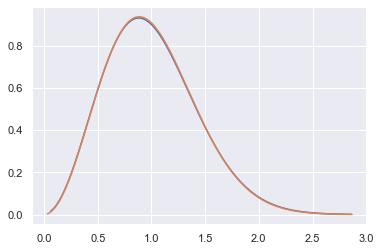
We can plot the density with Wigner's Surmise and see that Wigner's approximation is amazingly accurate, as expected from the experiments from last section.

Sampling from GUEs

We will now emperically verify our density curve. However, we will unfold the spectra using the procedure suggested by Andrew Odlyzko in The 10^20-th zero of the Riemann zeta function and 175 million of its neighbors. Suppose you have $n$ eigenvalues $\{ \lambda_i \}_{i=1}^n$, then the level spacings $\{ \mu_i \}_{i=1}^{n-1}$ can be normalized to have mean 1 by scaling the differences like so

$$\mu_i = (\lambda_{i+1} - \lambda_i)\frac{\sqrt{4n - \lambda_i^2}}{2 \pi}$$

Below we plot the level spacings for $200 \times 200$ GUE and compare the emperical distribution with the density curve found earlier.

Distribution of Spacings of $\zeta$

The Riemann zeta function is defined as the analytic continuation of the series

$$\zeta(s) = \sum_{n=1}^{\infty} \frac{1}{n^s} $$

where $s$ is a complex variable. The function satifies the following functional equation

$$\zeta(s) = 2^s \pi^{s-1} \sin(\frac{s \pi}{2}) \Gamma(1-s) \zeta(1-s) $$

Note that if $s$ is a negative, even integer then $\sin(\frac{s \pi}{2}) = 0 \Rightarrow \zeta(s) = 0$. The same cannot be said about positive even integers because of the poles of the Gamma function. Negative, even integers are known as the trivial zeros of the Riemann zeta function. The Riemann hypothesis states that the non-trivial zeros of the zeta function have real part $\frac{1}{2}$. This hypothesis remain unproven today and is one of the most famous open problems in mathematics. Andrew Odlyzko computed hundreds of examples of non-trivial zeros on his website, which we will use in this section. It turns out that there is a connection between Random Matrix theory and the non-trivial zeros of the Riemann zeta function. The differences of normalized imaginary non-trivial zeros of the Riemann zeta function follows the same distribution as the normalized level spacings of eigenvalues of GUE matrices. In particular, if $s_0$ is a non-trivial zero and $\Im(s_0) = \gamma$, we can normalize these gammas to have mean 1 with the following scaling

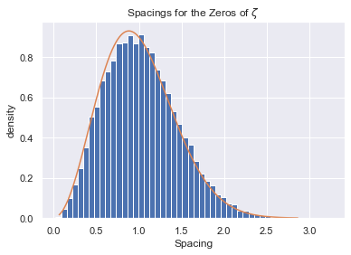
$$\tilde{\gamma} = \gamma \frac{1}{2 \pi} \log(\frac{\gamma}{2 \pi})$$

Below we import Odlyzko's data, normalize it, compute the differences, and plot it against the density curve found earlier in the section.