
from sympy import *
import numpy as np
from sympy import symbols, Function, integrate, diff
from scipy.special import airy
from scipy.integrate import solve_ivp, quad
import matplotlib.pyplot as plt
import seaborn as sns
import random

import sys
sys.path.append('../../')
import RandomMatrix as RM

%matplotlib inline
sns.set()

np.random.seed(140)
random.seed(140)
The Tracy-Widom distribution was defined by Craig A. Tracy and Harold Widom in their paper On Orthogonal and Symplectic Matrix Ensembles. It is an important distribution for studying the distribution of the fluctuations of the maximum eigenvalue of a Gaussian Ensemble. Each Gaussian ensemble has a corresponding Tracy Widom distribution. We will denote the Tracy Widom distribution for Gaussian Ensemble with Dyson index $\beta$ as $TW_\beta$. Let us study the distribution before its application.
Suppose $q$ is the solution to the Painlevé differential equation
$$q'' = sq + 2q^3 $$with the boundry condition $q \sim Ai(s)$ as $s \rightarrow \infty$. Define $I(t)$ and $J(t)$ to be the following
$$I(t) = - \int_{t}^{\infty} (x-t) q^2(x) dx$$$$J(t) = \int_{t}^{\infty} q(x) dx$$If we define $F_\beta$ to be the CDF of $TW_\beta$ then
$$F_2(t) = e^{I(t)}$$$$F_1(t) = \sqrt{F_2(t) e^{-J(t)}} $$To solve for the density of the Tracy Widom we would need to solve for a closed form solution to the Painlevé differential equation. We will instead approximate the curve using the Scipy's ODE solver. In order to define an initial condition, let $t_0$ be a large value so that the condition $q(t_0) = \text{Ai}(t_0)$ approximates our asymptotic boundry condition well. Using the Fundamental Theorem of Calculus, we can differentiate $I$ and $J$ to make them a solution to a differential equation our ODE solver can solve.
# Definition of I(t)
t, x = symbols("t x")
q = Function("q")
I = integrate((x-t)*q(x)**2, (x, t, oo))
I
# I'(t)
I_prime = diff(integrate((x-t)*q(x)**2, (x, t, oo)), t)
I_prime
# I''(t)
I_prime2 = diff(integrate((x-t)*q(x)**2, (x, t, oo)), t, 2)
I_prime2
Thus we can solve for $I(t)$ by solving for the differential equation
$$ \frac{d}{dt} \begin{pmatrix} \text{I}(t)\\ \text{I}'(t) \end{pmatrix} = \begin{pmatrix} \text{I}'(t)\\ q^2 \end{pmatrix} $$such that
$$I(t_0) = - \int_{t_0}^{\infty} (x-t_0) q^2(x) dx $$J = integrate(q(x), (x, t, oo))
J
# J'(t)
diff(J)
Thus we can solve for $J$ by solving
$$ \frac{dJ}{dt} = -q(t)$$such that
$$J(t_0) = \int_{t_0}^{\infty} q(x) dx$$In order to improve accuracy, we will use the solver to simultaneously find the values of $q(t)$, $I(t)$ and $J(t)$ in one system of differential equations. This strategy was suggested by Alan Edelman and Per-Olof Persson in their paper Numerical Methods for Eigenvalue Distributions of Random Matrices. Note that we must now slightly change our initial conditions for $I(t)$ and $J(t)$ to avoid using $q$ (since we won't have an approximation for it yet). Luckly, we decided to choose $t_0$ large enough so that $q(t) \approx \text{Ai}(t)$ for $t \geq t_0$, so we may replace $q$ in our intial conditions with $\text{Ai}$. The system of differential equations becomes
$$\frac{dy}{dt} = \begin{pmatrix} q' \\ tq+2q^3 \\ I' \\ q^2 \\ -q \end{pmatrix}$$where
$$y = \begin{pmatrix} q \\ q' \\ I \\ I' \\ J \end{pmatrix}$$such that
$$y(t_0) = \begin{pmatrix} \text{Ai}(t_0) \\ \text{Ai}'(t_0) \\ \int_{t_0}^{\infty} (x-t_0) \text{Ai}^2(x) dx \\ \text{Ai}(t_0)^2 \\ \int_{t_0}^{\infty} \text{Ai}(x) dx \end{pmatrix} $$Below we define the function we will pass into the ODE solver
def f(t, y):
    d0 = y[1]
    d1 = t*y[0]+2*y[0]**3
    d2 = y[3]
    d3 = y[0]**2
    d4 = -y[0]
    return np.array([d0, d1, d2, d3, d4])
Set the parameters
t0 = 4
tf = -6
Define the initial condition
y0_0 = airy(t0)[0]
y0_1 = airy(t0)[1]
y0_2 = quad(lambda x: (x-t0)*airy(x)[0]**2, t0, np.inf)[0]
y0_3 = airy(t0)[0]
y0_4 = quad(lambda x: airy(x)[0], t0, np.inf)[0]
y0 = np.array([y0_0, y0_1, y0_2, y0_3, y0_4])
Solve the ODE
sol = solve_ivp(f, (t0, tf) ,y0, max_step=.1)
Find the density of $TW_2$
F2 = np.exp(-sol.y[2])
f2 = -sol.y[3] * F2
Find the density of $TW_1$
F1 = np.sqrt(F2 * np.exp(-sol.y[4]))
f1 = 1/(2*F1)*(f2+sol.y[0]*F2)*np.exp(-sol.y[4])
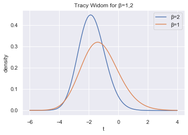
Plot the densities
plt.plot(sol.t, f2, label="β=2")
plt.plot(sol.t, f1, label="β=1")
plt.xlabel("t")
plt.ylabel("density")
plt.title("Tracy Widom for β=1,2")
plt.legend();
Tracy and Widom derived the distribution in their paper and proved its relationship to the fluctuations of the largest eigenvalue of Gaussian ensembles. Let the CDF for the $N \times N$ Gaussian ensemble with Dyson index $\beta$ be denoted as $F_{N, \beta}$. Also define $F_\beta$ and $f_\beta$ to be the CDF and density of the Tracy Widom distribution for Dyson index $\beta$ respectively. Tracy and Widom proved the following theorem
$$ F_\beta(s) = \lim_{N \rightarrow \infty} F_{N, \beta} \left(2 \sigma \sqrt{N} + \frac{\sigma s}{N^{1/6}} \right)$$We can take the derivative to find the density of the distribution
$$ \begin{align} \begin{aligned} f_\beta(s) &= \lim_{N \rightarrow \infty} f_{N,\beta} \left(2 \sigma \sqrt{N} + \frac{\sigma s}{N^{1/6}} \right) \frac{\sigma}{N^{1/6}} \\\\ &= \lim_{N \rightarrow \infty} f_{N, \beta} \left(\frac{s+2\sqrt{N}N^{1/6}}{\frac{N^{1/6}}{\sigma}} \right) \frac{1}{\frac{N^{1/6}}{\sigma}} \end{aligned} \end{align} $$Recall the formula for the density of linear transformations $f_{aX+b}(s) = f_{X}(\frac{s-b}{a}) \frac{1}{|a|}$. This implies that if $\lambda_{\max}$ is the greatest eigenvalue and $\sigma$ is the standard deviation of it's off diagonals, then
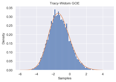
$$\lim_{N \rightarrow \infty} \frac{N^{1/6}}{\sigma} \lambda_{\max} - 2 \sqrt{N} N^{1/6} \sim \text{Tracy Widom}_{\beta}$$Recall from the first chapter the off diagonal terms in a GOE have standard deviation $\frac{1}{\sqrt{2}}$
trials = 10000
GOE_samples = []
N = 400
σ = 1/(np.sqrt(2))
for _ in range(trials):
    A = RM.Generate_GOE(N)
    λs = np.linalg.eigvals(A)
    λ_max = max(λs)
    GOE_samples.append(N**(1/6) * (λ_max/σ - 2*np.sqrt(N)))
plt.ylabel("Density")
plt.xlabel("Samples")
plt.title("Tracy-Widom GOE")
plt.hist(GOE_samples, bins=70, density=True)
plt.plot(sol.t, f1);
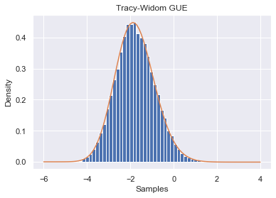
Recall from the first chapter that the off diagonal terms of a GUE have standard deviation 1.
trials = 30000
GUE_samples = []
N = 100
σ = 1
for _ in range(trials):
    A = RM.Generate_GUE(N)
    λs, V = np.linalg.eigh(A)
    λ_max = max(λs)
    GUE_samples.append(N**(1/6)*(λ_max/σ - 2*np.sqrt(N)))
plt.ylabel("Density")
plt.xlabel("Samples")
plt.title("Tracy-Widom GUE")
plt.hist(GUE_samples, bins=50, density=True)
plt.plot(sol.t, f2);
The Tracy Widom distribution suprisingly arises when studying sequences, as explained in On the Distribution of the Length of the Longest Increasing Subsequence of Random Permutations by Jinho Baik, Percy Deift, and Kurt Johansson. Let $S_N$ be the group of permutations of $1,2,3,...,N$. Define $\ell_N(\pi)$ to be the longest monotone increasing subsequence $\pi \in S_n$. Then
$$ \frac{\ell_N - 2\sqrt{N}}{N^{1/6}} \longrightarrow TW_2$$as $N \longrightarrow \infty$.
Below we sample from $S_N$, measure their lengths and plot the normalized distribution where $N=5000$.
def longest_increasing_subsequence(X):
    # https://en.wikipedia.org/wiki/Longest_increasing_subsequence#Efficient_algorithms
    """Returns the Longest Increasing Subsequence in the Given List/Array"""
    N = len(X)
    P = [0] * N
    M = [0] * (N+1)
    L = 0
    for i in range(N):
        lo = 1
        hi = L
        while lo <= hi:
            mid = (lo+hi)//2
            if (X[M[mid]] < X[i]):
                lo = mid+1
            else:
                hi = mid-1
        newL = lo
        P[i] = M[newL-1]
        M[newL] = i
        if (newL > L):
            L = newL
    return L

def sample_random_perm_lens(N, sample_size):
    lengths = []
    numbers = np.arange(1, N+1)
    for _ in range(sample_size):
        random.shuffle(numbers)
        lengths.append(longest_increasing_subsequence(numbers))
    return lengths
N = 5000
sample_size = 10000
perm_lens = sample_random_perm_lens(N, sample_size)
χ = (perm_lens - 2*np.sqrt(N))/N**(1/6)
plt.hist(χ, bins=28, density=True)
plt.plot(sol.t, f2, label="β=2");
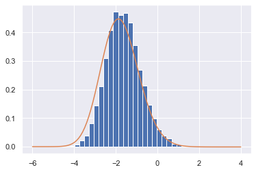
We expect the bias to be corrected as we increase $N$, but that may be very computationally expensive.