Joint Probability Density

The joint probability density of the eigenvalues (in no particular order) for an $N \times N$ gaussian ensemble with Dyson index $\beta$ is given by

$$f(\lambda_1, ... , \lambda_n) = \frac{1}{Z_{N,\beta}} e^{\left(-\frac{1}{2} \sum_{i=1}^N \lambda_i^2 \right)} \prod_{j<k} |\lambda_j - \lambda_k|^\beta $$

where

$$Z_{N,\beta} = (2\pi)^{N/2} \prod_{k=1}^N \frac{\Gamma(1+k\frac{\beta}{2})}{\Gamma(1+ \frac{\beta}{2})}$$

The RandomMatrix package has this density implemented as the gaussian_ensemble_density function. Below we calculate the joint density of a $2 \times 2$ GOE ($\beta=1$) for eigenvalues $1$ and $-1$.

We can create a heatmap of the density. First for the sake of computational efficiency, we will create the joint density function for the special case of $2 \times 2$ Gaussian Ensembles.

We can verify this function gives the same answer as the RandomMatrix package.

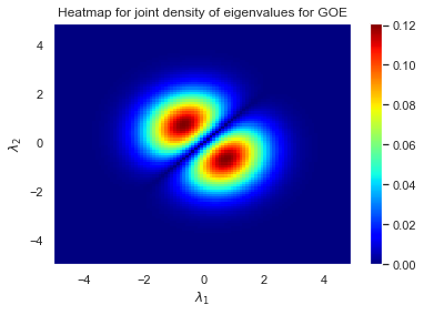
Now we can use this function to create a heatmap for $\beta=1$.

Emperical Experiment

We can create an emperical heatmap by generating GOEs and plotting a heatmap of it's eigenvalues.

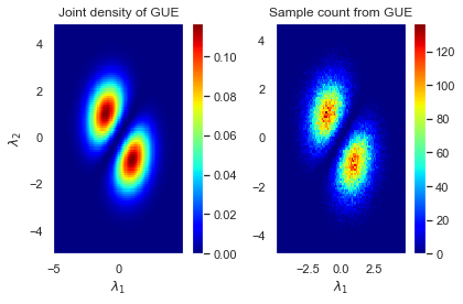
We can try the same exercise for GUEs and plot the actual joint density next to the emperical one for comparison.

$\beta$-Hermite Matrix

Ioana Dumitriu and Alan Edelman wrote an influencial paper Matrix Models for Beta Ensembles introduced a new method of sampling from Gaussian Ensembles. Define the $\beta$-Hermite matrix of size $n \times n$ as follows

$$ H_{\beta} \sim \frac{1}{\sqrt{2}} \begin{pmatrix} N(0,2) & \chi_{(n-1)\beta} & 0 & \cdots & 0\\ \chi_{(n-1)\beta} & N(0,2) & \chi_{(n-2)\beta} & \cdots & 0 \\ 0 & \chi_{(n-2)\beta} & N(0,2) & \ddots & 0 \\ \vdots & \vdots & \ddots & \ddots & \chi_{\beta} \\ 0 & 0 & \cdots & \chi_\beta & N(0,2) \end{pmatrix} $$

The eigenvalues of this real, tridiagonal matrix is equal in distribution to the eigenvalues of the $\beta$-Gaussian ensemble. The Generate_Hermite function in the RandomMatrix library will sample a hermite matrix. If we wanted to sample eigenvalues from GUEs, we could generate a $2$-Hermite matrix and find its eigenvalues. Below we recreate the heatmap for the joint density of the eigenvalues for a $2 \times 2$ GUE using the Generate_Hermite function.

Ghosts and Shadows

In The Random Matrix Technique of Ghosts and Shadows, Alan Edelman explains how the Gaussian ensemble can be studied in a more 'general' sense by allowing the Dyson index to be any positive, real number. This idea is very abstract when one realizes it doesn't make much sense to say that $\beta=1.5$ since that would imply the algebra has 1.5 dimension over the reals. This requires us to allow random matrix ensembles that can't be sampled. Edelman calls these objects ghost random matrices. A real or complex quantity from these ghosts that can be sampled or computed are called shadows. So although we can't sample ghosts, we can study their behavior through shadows.

For example, if $G_1, G_2, G_3, G_4$ are iid standard normal variables then

$$x_1 := G_1 \Rightarrow |x_1| = \sqrt{G_1^2} \sim \chi_1 $$$$x_2 := G_1 + iG_2 \Rightarrow |x_2| = \sqrt{G_1^2 + G_2^2} \sim \chi_2$$$$x_4 := G_1 + iG_2 + jG_3 + kG_4 \Rightarrow |x_4| = \sqrt{\sum_{i=1}^4 G_i} \sim \chi_{4}$$

Each of the $x_i$s above correspond to a one of the real division algebras ($\mathbb{R}, \mathbb{C}, \mathbb{H}$). Note that in all cases, $|x_\beta| = \chi_\beta$. If we wanted to define a ghost $x_\beta$ for any $\beta > 0$, we wouldn't be able to sample such an $x$ unless $\beta=1,2,4$ by the Frobenius theorem of real division algebras. We could however sample the shadow of $|x_\beta|$ by simply sampling from the $\chi_\beta$ distribution. This works beause the degrees of freedom parameter for the chi-distribution can be any strictly positive real number.

Note that if we wanted to study matrices of a $\beta$-Gaussian ensemble, we could use the $\beta$-Hermite matrix above as a shadow! So although it is impossible to sample a $\beta=1.5$ Gaussian matrix, we are able to sample its eigenvalues from its ghost.